Utilizing Optimal F in Scenario Planning
I am a huge fan of the portfolio allocation frameworks developed by Ralph Vince. I own all of his books.
- Portfolio Management Formulas
- The Mathematics of Money Management
- The Handbook of Portfolio Mathematics
- The New Money Management
- The Leverage Space Trading Model
- Risk-Opportunity Analysis
His work has done much to inspire me. I have tested most of his formulas extensively and have found the results to be fascinating.
Nevertheless, there is a concept which was mentioned in his book The New Money Management that I have always wanted to explore further. It has to do with utilizing Optimal f equations in a scenario planning environment.
For those of you not familiar with either optimal f or scenario planning, a brief primer is in order. I will attempt to keep it as short as possible.
Background on Optimal f
The thesis behind Ralph’s work is really an extension of the Kelly criterion. It turns out that trading in the markets by utilizing the Kelly criterion is difficult due to the fact the Kelly equations demand for wins and losses to be the exact same amount, just different sign conventions. In a system (such as life, trading markets, etc.) wins and losses are rarely of the same amount, thus a framework had to be developed in order to calculate the optimal fractional bet size given these parameters.
The Optimal f equations aid us in one goal. Discovering the fractional amount of one’s entire capital which they should place on each bet given a statistical outcome. Over time, if the statistical outcome remains steady and does not change, betting the Optimal f amount will be the fastest way to maximizing one’s capital.
It is important to note for Optimal f to work, several items must be present.
- A game in which there is a positive mathematical expectation.
- A game where the statistical outcomes stay steady, or at least don’t drop the game into a negative mathematical expectation.
- A game where wins and losses can be tracked and enumerated in real values.
- A game where the capital is large enough to take fractional stakes.
- A game where the frequency is large enough for the effect of optimal f can be realized.
That list doesn’t appear difficult. Any equity, commodity, or forex market meets all of the above criteria…almost. The only difficult part is finding a trading strategy which possesses a positive mathematical expectation and stays positive long enough to work the optimal f equations upon.
Many firms sell such “backtested” strategies, but the markets are always changing. It is way more difficult than it appears.
Background on Scenario Planning
I am going to borrow some of Ralph’s language here. The world of forecasting is complicated. As humans, we tend towards being too optimistic when forecasting outcomes. To compound that problem, we usually like to forecast only the most probable outcome. This obviously leads to problems given the fact certainty is a grand illusion. It would be much better for us to think in terms of all possible scenarios which might occur tomorrow given the facts we have today.
Once we are in position of such scenarios, we can then create plans for each of the probable outcomes.
However, we can go further than that.
We can also assign probabilities of occurrence to these different scenarios. Taking our assessment one step beyond, we can also assign amounts of positive or negative gain to each scenario as well. Given this information, we would then be able to exercise our Optimal f equations on our scenario matrix.
Assigning Probabilities
Assigning probabilities to certain scenarios may be one of the most difficult aspects of forecasting. Nevertheless, there are very easy methods to utilize in order to assist us with this adversity. I always like to turn to the “Wisdom of Crowds” method. It has proven to be most robust in my career and it’s actually been extremely accurate.
You are familiar with the concept. Have you ever seen a contest at a local fair or fall festival where everyone was asked to bet on the number of jelly beans in the jar? Obviously, the guesses would be vary greatly, but the actual average of all of them would be quite close to the amount inside the jar. It’s the power of the collective brain, so to speak. Over the past two decades, there has been much research on the impact of knowing other people’s guesses and how it affects the outcome. Until that research proves conclusive, I would always encourage those who need to utilize this method to do so in a blind way.
Ralph’s Example
I’m going to attempt to duplicate Ralph’s example inside of his book just to make sure that all of our equations and code are working correctly. In his book, The New Money Management, on page 49, Ralph presents us with an example of a business case. We are told that XYZ Corporation is needing to make a decision on how much to allocate towards marketing a new product in a remote country.
In his example, we are given five separate scenarios. Obviously, we could be utilizing more in this methodology, but 5 works just fine for our purposes.
He also assigns probabilities and financial results to each scenario.
We are given a table that looks something like this.
| Scenario | Probability | Result |
|---|---|---|
| War | 0.1 | -$500,000 |
| Trouble | 0.2 | -$200,000 |
| Stagnation | 0.2 | 0 |
| Peace | 0.45 | $500,000 |
| Prosperity | 0.05 | $1,000,000 |
Next we are instructed to utilize the following equation to discover our Optimal f given these scenarios. Here’s equation 1.22 found on page 45.
\[G=\left(\prod\limits_{i=1}^T\left(\left(1 +\left(\frac{A_i}{\left(\frac{W}{-f}\right)}\right)\right)^{P_i}\right)\right)^{1/\sum_{p_i}}\]
Then on page 52 we are given the results and their interpretation. We’re shown that the Optimal f value in this instance would be 0.57, G = 1.1106, and company XYZ should allocate $877,192.35 into their marketing campaign. This dollar figure is arrived at by dividing the worst possible scenario by the negative value of Optimal f.
Let’s recreate this problem in Python and see if we can come up with the same results!
           #!/usr/bin/env python3

           import numpy as np
           import pandas as pd
           import matplotlib.pyplot as plt
           from decimal import Decimal, getcontext

           getcontext().prec = 8

           amounts = [-500000, -200000, 0.0, 500000, 1000000]
           probabilities = [0.1, 0.2, 0.2, 0.45, 0.05]
           outcome = ["War", "Trouble", "Stagnation", "Peace", "Prosperity"]

           total_sum = sum(amount * prob for amount, prob in zip(amounts, probabilities))
           W = min(amounts)
           print("Total sum to check for postive mathematical expectation:", total_sum)
           print(W)

           results = []

           for i in np.arange(0.01, 1.01, 0.01):
               cumulative_product = 1
               for amount, prob in zip(amounts, probabilities):
                   result = ((amount / (W / -i)) + 1) ** prob
                   cumulative_product *= result

               results.append({'f': i, 'TWR': cumulative_product})

           df = pd.DataFrame(results)

           print(df.iloc[df['TWR'].idxmax()])
           max_twr_row = df.iloc[df['TWR'].idxmax()]
           optimal_f = Decimal(max_twr_row['f']).quantize(Decimal('0.01'))
           print("Optimal f:", optimal_f)
           optimal_amount = W / - optimal_f
           print(f"The Optimal amount to invest is :${optimal_amount:.2f}")

           filtered_df = df[df['TWR'] > 1.0]
           plt.figure(figsize=(10, 6))
           plt.plot(filtered_df['f'], filtered_df['TWR'], marker='o', linestyle='-')
           plt.xlabel('f')
           plt.ylabel('TWR')
           plt.title('Ralphs Scenario Planning Example')
           plt.grid(True)
           plt.show()
A few important notes before we see our terminal output and plot. You may notice I have left the output labeled as TWR (Total Wealth Relative) and not G. This is so I can denote in the code at a later date I have not utilized the entire equation. If you will notice when we raise everything to the power of 1 divided by the summation of our probabilities, that entire term falls to 1, which renders it useless.
Now for our terminal output.
           Total sum to check for postive mathematical expectation: 185000.0
           -500000
           f      0.57000
           TWR    1.11057
           Name: 56, dtype: float64
           Optimal f: 0.57
           The Optimal amount to invest is :$877192.98
YES! I did it! Everything matches exactly…well I guess I am off by $0.63…but I will take it. All of our results here match with everything presented in Ralph’s example. Let’s take a look at the plot.
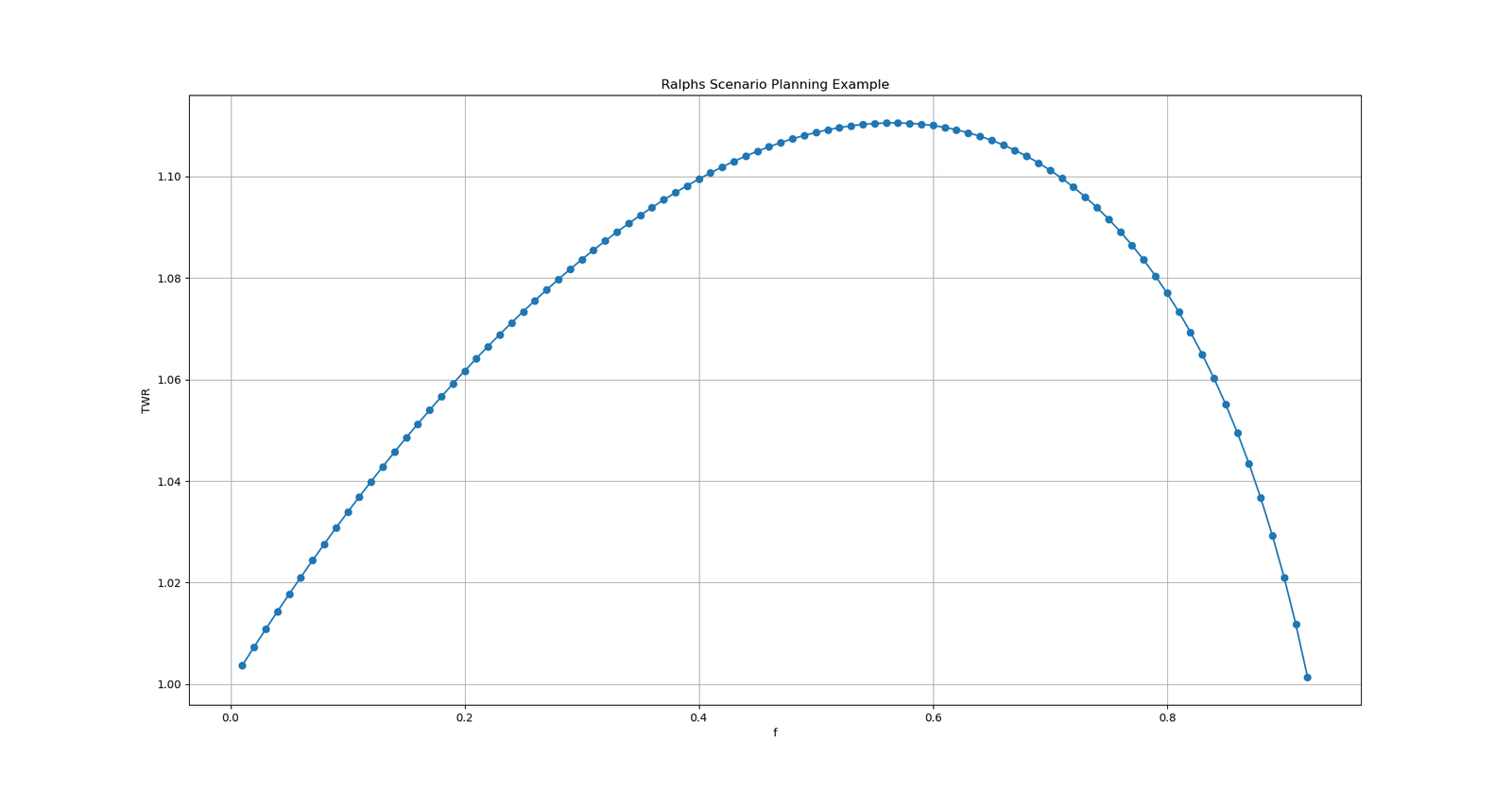
As you can see, everyone is somewhere on the f curve, if you don’t know where your maximum is, you are only cheating yourself.
Jonathan’s Example
How exciting. Now with this tool under our belts, we can do all sorts of magic consulting for businesses both large and small. Let’s make up our own example and use the exact same code, just with some different values and take a look at the results. What fun!
Imagine this. I get a call from Shoe Carnival (It is one of my favorite companies) and they ask me to come up to Evansville and do a little consulting. I happily oblige.
They are contemplating making an investment in some new AI technology this quarter. Let’s say it helps with their inventory tracking. The vendor of the AI technology offers the product in three different tiers or price points.
- Base Package $4.7 Million
- Gold Package $6.9 Million
- Deluxe Package $11.8 Million
They have to make a decision tomorrow morning. There is no time to collect data for six months, no time for research. The decision needs to be made now. The only hard number they have been given to go off of is if they purchase the deluxe package, they can make an additional $14.9 Million dollars of profit, even after having covered the investment cost.
First, let’s come up with scenarios and assign dollar amounts to each.
Scenario 1
We will call this a “Total Loss.” They invest the $11.8 Million into this new AI Technology and receive absolutely zero return.
Scenario 2
We will label this scenario, “Less Loss.” In this instance, they will invest $11.8 million but makes up enough profit where they only lose $4.7 million.
Scenario 3
Here they will be investing $11.8 million and making back $11.8 million. Thus, their final profit will be absolutely zero. No loss, but no gain.
Scenario 4
We will label this scenario “Increased Revenue.” here we’re going to make back our investment plus an additional 4.8 million dollars
Scenario 5
This will be our best case and we’re going to label it “Outstanding.” In this scenario, Shoe Carnival will actually make a profit of $14.9 million by investing in this new AI technology.
Now we really have something to work with. However, we are still missing our probabilities. Let’s utilize the “Wisdom of Crowds” methodology in order to assign these probabilities to each scenario. We have three long-term executives in this room. There’s quite a bit of knowledge here.
I simply ask each executive to write on a sheet of paper what they think the probability of each scenario occurring is. They can assign any value they like, The total doesn’t even have to add up to be 100%. Now I simply take the average of each person’s vote across each scenario utilizing a simple average formula.
\[{\displaystyle {\bar {p}}={\frac {1}{n}}\left(\sum _{i=1}^{n}{p_{i}}\right)={\frac {p_{1}+p_{2}+\dots +p_{n}}{n}}}\]
At this point, I’ll be left with something that looks like this.
- Scenario 1 = 21.7%
- Scenario 2 = 21.7%
- Scenario 3 = 43.4%
- Scenario 4 = 104.16%
- Scenario 5 = 26.04%
Don’t be alarmed that these percentages add up to be greater than 100%. We will simply weigh them against their summation in order to bring down the percentages to a 100% standard. The summation of all of our probabilities is equal to 217%. Now, by dividing each scenario probability by that number, we will arrive at decimal equivalents, the sum of which will equal 1. Exactly what we want.
Given all this information, we can create our own table which will look like this.
| Scenario | Probability | Result |
|---|---|---|
| Total Loss | 0.1 | -$11,800,000 |
| Less Loss | 0.1 | -$4,700,000 |
| Nothing | 0.2 | 0.0 |
| Increased Revenue | 0.48 | $4,800,000 |
| Outstanding | 0.12 | $14,000,000 |
We now have everything we need. Let’s plug these numbers into our Python code and see what happens.
           #!/usr/bin/env python3

           import numpy as np
           import pandas as pd
           import matplotlib.pyplot as plt
           from decimal import Decimal, getcontext

           getcontext().prec = 8

           amounts = [-11800000, -4700000, 0.0, 4800000, 14900000]
           probabilities = [0.1, 0.1, 0.2, 0.48, 0.12]
           outcome = ["Total Loss", "Less Loss", "Nothing", "Increased Revenue", "Outstanding"]

           total_sum = sum(amount * prob for amount, prob in zip(amounts, probabilities))
           W = min(amounts)
           print("Total sum to check for postive mathematical expectation:", total_sum)
           print(W)

           results = []

           for i in np.arange(0.01, 1.01, 0.01):
               cumulative_product = 1
               for amount, prob in zip(amounts, probabilities):
                   result = ((amount / (W / -i)) + 1) ** prob
                   cumulative_product *= result

               results.append({'f': i, 'TWR': cumulative_product})

           df = pd.DataFrame(results)

           print(df.iloc[df['TWR'].idxmax()])
           max_twr_row = df.iloc[df['TWR'].idxmax()]
           optimal_f = Decimal(max_twr_row['f']).quantize(Decimal('0.01'))
           print("Optimal f:", optimal_f)
           optimal_amount = W / - optimal_f
           print(f"The Optimal amount to invest is :${optimal_amount:.2f}")

           filtered_df = df[df['TWR'] > 1.0]
           plt.figure(figsize=(10, 6))
           plt.plot(filtered_df['f'], filtered_df['TWR'], marker='o', linestyle='-')
           plt.xlabel('f')
           plt.ylabel('TWR')
           plt.title('SCVL Scenario Planning Example')
           plt.grid(True)
           plt.show()
Let us first check our plot to make sure everything is looking good.

Now for the terminal output:
           Total sum to check for postive mathematical expectation: 2442000.0
           -11800000
           f      0.510000
           TWR    1.057704
           Name: 50, dtype: float64
           Optimal f: 0.51
           The Optimal amount to invest is :$23137255.00
Hold Up - We have a problem!
In Ralph’s example, we were given at least one outcome which was greater than the optimal amount we were to invest. However, in the case of our Shoe Carnival example, our optimal investment amount is much greater than any possible return we could receive. What does this mean?
It would appear that optimal f actually fails when utilized in a scenario planning application given these equations. Under no circumstances would any business be expected to invest $23,137,255 for just a chance of making $14,900,000.
Should we throw out optimal f and treat it as a failure? Absolutely not. I am convinced of the validity of Mr. Vince’s work under every other presentation which he has made. However, in this instance, something is incorrect. I suspect the problem lies within the interpretation of the optimal f values under the scenario planning case, or within the calculation of the HPRs via the raising of the inner term to the power of the individual scenario probability.
Sadly, the time I am allowed to allocate to this project is coming to an end. My hope was to present to you a fascinating tool which could be utilized to find optimal amounts of investment in different scenarios. Given these issues I’m going to be unable to make that claim.
I hope I will get a chance to revisit this work and see if I can’t find where the problem is. If you have any suggestions, please feel free to contact me. I’ll be very interested in hearing your thoughts.
Jonathan Adams
August 4th, 2025